Uniform Sampling on Disks, Shells, Balls, and Triangles.
Table of Contents
Overview
Uniform sampling of an arbitrary geometry is a common task that you might encounter in your
research. This post summarizes the general inverse approach. I learned the approach in the classic
PBRT book, which is one of my favorite books even beyond computer graphics.
Methods
We start with the basics of sampling a 3D hemisphere shell that is parameterized in the polar
coordinate:
- We need to find \(p(\theta, \phi)\) so that if we take a sample from this distribution, we are
sampling uniformly from the hemisphere.
- We then run use the inverse transform sampling method to sample \(\theta\) from \(p(\theta)\) and \(\phi \sim
p(\phi \mid \theta)\) with the given \(\theta\).
How do we find \(p(\theta, \phi)\) in the first place? We need to understand that if we are
sampling uniformly from a geometry, then
\[p(\theta, \phi)\mathrm{d}\phi \mathrm{d}\theta \propto \mathrm{d}A. \tag{1}\]
This is saying that \(p(\theta, \phi)\mathrm{d}\phi \mathrm{d}\theta\) must be proportional
to the area or volume of the infinitesimal region \(\mathrm{d}A\) on the geometry. If this holds,
then two infinitesimal regions with the same area will be sampled with equal probability.
Once Equation (1) is crystal clear to you, the rests are just math manipulation. We will derive
the result on 2D disks, 3D sphere surfaces, and balls.
1. 3D Hemisphere Shells
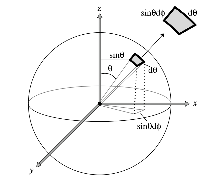
To derive the \(\mathrm{d}A\) for a hemisphere, it is important to understand Figure 1:

Figure 1. Infinitesimal
area of a hemisphere.
For the infinitesimal area, it is obvious that one side is \(\mathrm{d}\theta\). For the other
side, you need to pay attention to its projection on the horizontal plane. The projected arc has
radius of \(\sin\theta\) and radian of \(\mathrm{d}\phi\). Assuming \(r=1\), we have
\[\mathrm{d}A = \sin\theta\mathrm{d}\phi\mathrm{d}\theta,\]
which gives
\[p(\theta, \phi) \propto \sin\theta.\]
For \(\phi\), it can be drawn from uniform distribution \(\phi \sim U(0, 2\pi)\) which is trivial.
For \(\theta\), we compute its CDF:
\[P(\theta) = \int_0^{\theta} \sin\theta' \mathrm{d}\theta' = 1-\cos\theta. \]
With the inverse sampling approach, we have
\[
\begin{align}
\theta &= \cos^{-1}(1-\xi_1) = \cos^{-1}\xi_1' \\
\phi &= 2\pi\xi_2
\end{align}
\]
where \(\xi_1',\xi_2\) are randomly sampled from $[0,1]$.
2. 3D Hemisphere Volume
Similar to the hemisphere shell, we have the volume infinitesimal
\[\mathrm{d}V = r^2\sin\theta\mathrm{d}r\mathrm{d}\phi\mathrm{d}\theta,\]
which gives
\[p(r, \theta, \phi) \propto r^2\sin\theta.\]
This gives \(p(r) \propto r^2\) and \(p(\theta\mid r) \propto \sin\theta\). We can compute the
CDF of \(p(r)\):
\[P(r) \propto \int_0^{r} r'^2 \mathrm{d}r' \propto r^3 \]
With the inverse sampling approach, we have
\[
\begin{align}
r &= \sqrt[3]{\xi_0} \\
\theta &= \cos^{-1}\xi_1' \\
\phi &= 2\pi\xi_2
\end{align}.
\]
3. 2D Disks
Sampling 2D disk can be derived similarly to the 3D ball case. The results are
\[
\begin{align}
r &= \sqrt[2]{\xi_0} \\
\phi &= 2\pi\xi_2
\end{align}.
\]
4. 2D Triangles
To sample on 2D triangles, we use the barycentric coordinate \((u, v)\) such that \(0 \le u+v\le 1\) and \(0 \le u,v\le 1\). Since it is a flat
surface, it is obvious that
\[
p(u, v) \propto c.
\]
Therefore, we have
\[
\begin{align}
p(u) &\propto \int_{0}^{1-u} c \mathrm{d}v \propto 1-u\\
p(v \mid u) &= \frac{p(u,v)}{p(u)} \propto \frac{1}{1-u}
\end{align}.
\]
The CDFs are
\[
\begin{align}
P(u) &= 2u-u^2\\
p(v \mid u) &\propto v = \frac{v}{1-u}
\end{align}.
\]
Assign the CDFs to uniform distributed random numbers and solve a quadratic equation, we have
\[
\begin{align}
u &= 1 - \sqrt{1-\xi_1} \\
v &= \xi_2\sqrt{1-\xi_1}
\end{align}.
\]
Overview
Uniform sampling of an arbitrary geometry is a common task that you might encounter in your research. This post summarizes the general inverse approach. I learned the approach in the classic PBRT book, which is one of my favorite books even beyond computer graphics.
Methods
We start with the basics of sampling a 3D hemisphere shell that is parameterized in the polar coordinate:
- We need to find \(p(\theta, \phi)\) so that if we take a sample from this distribution, we are sampling uniformly from the hemisphere.
- We then run use the inverse transform sampling method to sample \(\theta\) from \(p(\theta)\) and \(\phi \sim p(\phi \mid \theta)\) with the given \(\theta\).
How do we find \(p(\theta, \phi)\) in the first place? We need to understand that if we are sampling uniformly from a geometry, then
\[p(\theta, \phi)\mathrm{d}\phi \mathrm{d}\theta \propto \mathrm{d}A. \tag{1}\]
This is saying that \(p(\theta, \phi)\mathrm{d}\phi \mathrm{d}\theta\) must be proportional to the area or volume of the infinitesimal region \(\mathrm{d}A\) on the geometry. If this holds, then two infinitesimal regions with the same area will be sampled with equal probability.
Once Equation (1) is crystal clear to you, the rests are just math manipulation. We will derive the result on 2D disks, 3D sphere surfaces, and balls.
1. 3D Hemisphere Shells
To derive the \(\mathrm{d}A\) for a hemisphere, it is important to understand Figure 1:

For the infinitesimal area, it is obvious that one side is \(\mathrm{d}\theta\). For the other side, you need to pay attention to its projection on the horizontal plane. The projected arc has radius of \(\sin\theta\) and radian of \(\mathrm{d}\phi\). Assuming \(r=1\), we have
\[\mathrm{d}A = \sin\theta\mathrm{d}\phi\mathrm{d}\theta,\]
which gives
\[p(\theta, \phi) \propto \sin\theta.\]
For \(\phi\), it can be drawn from uniform distribution \(\phi \sim U(0, 2\pi)\) which is trivial. For \(\theta\), we compute its CDF:
\[P(\theta) = \int_0^{\theta} \sin\theta' \mathrm{d}\theta' = 1-\cos\theta. \]
With the inverse sampling approach, we have
\[ \begin{align} \theta &= \cos^{-1}(1-\xi_1) = \cos^{-1}\xi_1' \\ \phi &= 2\pi\xi_2 \end{align} \]
where \(\xi_1',\xi_2\) are randomly sampled from $[0,1]$.
2. 3D Hemisphere Volume
Similar to the hemisphere shell, we have the volume infinitesimal
\[\mathrm{d}V = r^2\sin\theta\mathrm{d}r\mathrm{d}\phi\mathrm{d}\theta,\]
which gives
\[p(r, \theta, \phi) \propto r^2\sin\theta.\]
This gives \(p(r) \propto r^2\) and \(p(\theta\mid r) \propto \sin\theta\). We can compute the CDF of \(p(r)\):
\[P(r) \propto \int_0^{r} r'^2 \mathrm{d}r' \propto r^3 \]
With the inverse sampling approach, we have
\[ \begin{align} r &= \sqrt[3]{\xi_0} \\ \theta &= \cos^{-1}\xi_1' \\ \phi &= 2\pi\xi_2 \end{align}. \]
3. 2D Disks
Sampling 2D disk can be derived similarly to the 3D ball case. The results are
\[ \begin{align} r &= \sqrt[2]{\xi_0} \\ \phi &= 2\pi\xi_2 \end{align}. \]
4. 2D Triangles
To sample on 2D triangles, we use the barycentric coordinate \((u, v)\) such that \(0 \le u+v\le 1\) and \(0 \le u,v\le 1\). Since it is a flat surface, it is obvious that
\[ p(u, v) \propto c. \]
Therefore, we have
\[ \begin{align} p(u) &\propto \int_{0}^{1-u} c \mathrm{d}v \propto 1-u\\ p(v \mid u) &= \frac{p(u,v)}{p(u)} \propto \frac{1}{1-u} \end{align}. \]
The CDFs are
\[ \begin{align} P(u) &= 2u-u^2\\ p(v \mid u) &\propto v = \frac{v}{1-u} \end{align}. \]
Assign the CDFs to uniform distributed random numbers and solve a quadratic equation, we have
\[ \begin{align} u &= 1 - \sqrt{1-\xi_1} \\ v &= \xi_2\sqrt{1-\xi_1} \end{align}. \]